What Is Linear Programming? Optimization Inside a Box of Constraints

Linear programming is the math behind airline ticket prices, shipping routes, and whether your factory builds 30 tables or 40 chairs this week. It almost never shows up on LeetCode. But if you want to know why max-flow min-cut is true rather than just memorizing it, LP is the explanation that makes it click. And if you want to sound about 40% smarter the next time you explain flow algorithms, this is the piece to read.

Three Ingredients, One Formula

Linear programming finds the maximum (or minimum) of a linear function subject to a set of linear constraints.

Three ingredients:

Decision variables. The things you control. Tables to build, packets to route, amount of each ingredient to mix.
Objective function. A linear combination of those variables you want to maximize or minimize.
Constraints. Linear inequalities that fence in what is feasible. Budget caps, capacity ceilings, non-negativity requirements.

"Linear" means no x², no xy, no absolute values. Every term is a constant times a variable. That restriction is exactly what makes LP tractable. The second you let things curve, you are in a different and considerably worse world.

A Concrete Example: The Factory Problem

You run a factory. Two products: tables and chairs.

Each table needs 4 carpentry hours and 2 painting hours. Profit: $180.
Each chair needs 3 carpentry hours and 1 painting hour. Profit: $120.
Available per week: 240 carpentry hours, 100 painting hours.

How many of each should you build? You could guess. Or you could just solve the LP.

Let x₁ = tables, x₂ = chairs.

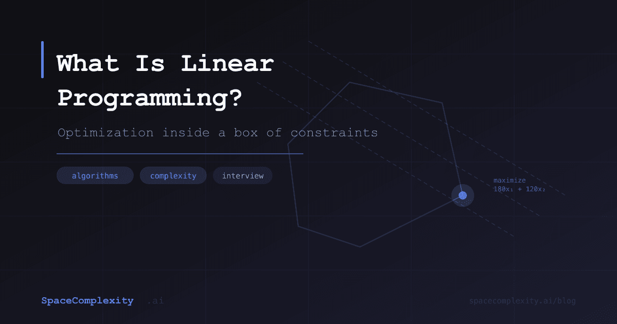
Maximize:    180·x₁ + 120·x₂

Subject to:  4·x₁ + 3·x₂ ≤ 240    (carpentry)
             2·x₁ +   x₂ ≤ 100    (painting)
                  x₁, x₂ ≥ 0

from scipy.optimize import linprog

c = [-180, -120]  # linprog minimizes, so negate
A_ub = [[4, 3], [2, 1]]
b_ub = [240, 100]

result = linprog(c, A_ub=A_ub, b_ub=b_ub, bounds=[(0, None), (0, None)])

print(f"Tables: {result.x[0]:.1f}, Chairs: {result.x[1]:.1f}")
print(f"Max profit: ${-result.fun:.0f}")
# Tables: 30.0, Chairs: 40.0
# Max profit: $10200

30 tables, 40 chairs, $10,200. No guessing, no gradient descent, no training data. Just math.

Why the Answer Is Always at a Corner

In two dimensions, each constraint cuts the plane in half. Together they carve out a convex polygon: the feasible region. Every point inside is a valid solution.

Your intuition probably says the optimum should be somewhere interior, safely away from all the constraint edges. Your intuition is wrong. The optimal always lives at a vertex of that polygon. Not somewhere in the middle. At a corner.

Here is why. The objective function 180x₁ + 120x₂ is a family of parallel lines, each representing a different profit level. Push that line upward and it slides across the feasible region. The last point it touches before leaving entirely is a corner. That corner is optimal.

This is the fundamental theorem of LP. You do not search an infinite space. You search the corners of a polytope. In higher dimensions the polytope has more corners, but the theorem holds.

The feasible region for the factory problem, with the optimal vertex highlighted where both constraints bind

Simplex: Walk the Corners

George Dantzig invented Simplex in 1947. The idea is almost embarrassingly simple. Start at any corner. Walk to an adjacent corner that improves the objective. Stop when no adjacent corner is better.

Each step is cheap: solve a small linear system. In practice, Simplex converges in steps proportional to the number of constraints, not the number of corners.

There is a catch. The Klee-Minty cube is a deliberately adversarial polytope that forces Simplex to visit all 2^n corners. Worst case is exponential. But this almost never happens with real data. Simplex remains the default in most LP solvers because in practice it is extremely fast. The Klee-Minty cube is a beloved theoretical gotcha that has scared exactly zero practitioners out of using Simplex.

Interior Point: Cut Through the Middle

The Klee-Minty cube exposed a theoretical weakness, not a practical one. But the question of whether LP was solvable in polynomial time in the worst case mattered to complexity theorists.

Leonid Khachiyan answered it in 1979 with the ellipsoid method: LP is in P. Polynomial, provably. The ellipsoid method was theoretically important and practically useless. Then Narendra Karmarkar came along in 1984 with an interior point method that actually worked. Instead of walking the boundary, it moves through the interior of the feasible region, scaling each step to stay well away from the constraints.

Interior point methods run in O(n^3.5 · L) time, where n is the number of variables and L is the input size in bits. Practically competitive with Simplex on most problems, and often better on very large instances. Modern solvers like HiGHS combine both.

Algorithm	Worst-Case	Notes
Simplex	O(2^n)	Adversarial only; fast in practice
Ellipsoid (Khachiyan)	O(n^6 L^2)	First poly-time proof; rarely used
Interior point (Karmarkar)	O(n^3.5 L)	Polynomial and practically fast

Space for all three is O(m · n), where m is the number of constraints.

Duality: Where Max-Flow Min-Cut Actually Comes From

Every LP has a corresponding dual LP. The dual of the maximization problem is a minimization problem with a symmetric structure. The strong duality theorem says both optimal values are equal when feasible solutions exist.

This is why max-flow equals min-cut. The max-flow problem can be written as an LP. Its dual is exactly the min-cut problem. Strong duality gives you the equality for free. The theorem is not a coincidence someone stumbled across. It falls out of LP structure.

The same thing explains why shortest paths and bipartite matching have such clean theoretical properties. They are all LPs in disguise, and their duals happen to be the problems you naturally think of as their "opposites."

When Integers Appear, Everything Changes

Standard LP lets variables take any real value. Add the constraint that all variables must be integers and you get Integer Linear Programming (ILP).

ILP is NP-hard. Congratulations, your nicely solvable polynomial problem just became the permanent residence of branch-and-bound search trees. The convex polytope geometry breaks down entirely. You cannot just walk corners anymore, because integer points are not corners of anything in particular.

A common technique: solve the LP relaxation first (drop the integrality requirement), get a fractional solution, then use it as a bound for branch-and-bound search. Many approximation algorithms for NP-hard problems work exactly this way: relax the problem to a real-valued LP, get a fractional answer, then figure out how much you lose by rounding.

Some LP instances have a special structure where the relaxation automatically produces integer solutions without any rounding. The condition is total unimodularity: every square submatrix of the constraint matrix has determinant in {-1, 0, 1}. Network flow, bipartite matching, and shortest paths all have totally unimodular constraint matrices. That is the deeper reason these problems are polynomial-time solvable even when they look like they might require integer solutions.

The integer restriction is what separates easy from hard. Traveling Salesman with fractional routes is a polynomial LP. Require integer routes and it is NP-hard. Knowing where that line sits changes how you think about problem reductions.

What This Means for Coding Interviews

LP does not appear directly in FAANG-style coding interviews. You will not implement Simplex. But the mental model pays off in a few concrete ways.

Max-flow and LP are the same problem. When you reach for a flow algorithm, you are implicitly solving an LP. Knowing this helps you recognize flow structure in disguise and understand why flow algorithms always terminate with integer solutions on integer-capacity graphs.

Greedy works when LP relaxations are integral. If a greedy algorithm solves an optimization problem correctly, the formal justification usually involves total unimodularity. Activity selection, interval scheduling, bipartite matching via augmenting paths: all work because the underlying LP already has integer vertices.

If you want to practice articulating this kind of complexity reasoning under pressure, SpaceComplexity runs live voice-based mock interviews where you have to explain not just the algorithm but why it works and where it breaks.